Tuesday 4 March 2014

Set Up Visual Studio 2012 for CUDA Dynamic Parallelism

In this post i am going to show you how to set up Visual Studio 2012 to compile CUDA code which uses dynamic parallelism.

What is Dynamic Parallelism?


Dynamic parallelism enables the GPU to create new work for itself without ever having to involve the CPU by allowing CUDA kernels to call other CUDA kernels.

Nvidia 2013
This is a powerful tool for CUDA developers as there is now no longer the need to pass data between the host and device as launch configuration decisions can now be made at runtime by threads executing on the device.

In order to make use of dynamic parallelism you must have an Nvidia GPU with compute capability 3.5

Dynamic Parallelism Example


As with every first code example we will look at a simple 'hello world' program which uses dynamic parallelism. 


Here we have two kernels, the parent kernel and the child kernel. Out parent kernel calls the child, waits for it to complete its work and then carries out some work of its own. 

When we initially try and build this code using visual studio we will get the following error. 


Visual studio is complaining that we can only call kernels within kernels if we have a card of compute 3.5 or higher. To let visual studio know that we do infact have a suitable card we need to change a few properties. 

To do this we open up the project properties by right clicking on the project. 


The first setting we need to change is to tell CUDA to generate relocatable device code by selecting 'Yes (-rdc=true)'


Next we have to tell CUDA to use compute 3.5 by changing the code generation to 'compute_35,sm_35'


We then need to tell the runtime library to use the multi threaded library. If we are in debug mode we select 'Multi-Threaded Debug (/MTd)' or if we are in release mode 'Multi-Threaded (/MT)'


Finally inside the linker properties we add an additional dependency to 'cudadevrt.lib' 

After following these steps our project will now build successfully and we should get the following output. 


This has been to mostly help remind myself how to set up visual studio in the future if i forget but hopefully it can help out a few other people as well. 

Any questions or if you are struggling with anything feel free to send me an email at craigmcmillan01@outlook.com with blog in the subject and i will be happy to help. 

Monday 27 January 2014

Global Game Jam 2014

So it was the global game jam this weekend and me and a few friends decided to team up and make a game over the 48 hours. The theme this year was the quote "We don't see things as they are, we see them as we are." 

From this we decided to make a first person tower defence game; you protect the gate to the town of Woodbury but you can't tell your enemies from your friends! Shine a light on them to reveal their true nature then take them out with your kick-ass crossbow! 

If you would like to play the game you can download a copy from the global game jam website or check out the video below.

You can also check out what the rest of the team have been up to as well.

Scott Ranken - Programmer
Leigh Norton - Programmer
Michael Norton - Programmer 


Tuesday 21 January 2014

Sequential Dijkstra

Some of the work i have carried out as part of my honours project can be found below. This post looks at a sequential implementation of Dijkstra's pathfinding algorithm.

10004794 Honours Project: Technical Work: Sequential Dijkstra:

Thursday 2 January 2014

Parallel IDEA Algorithm

For one of my coursework's this year we had to parallelize the International Data Encryption Algorithm using different CPU concurrency techniques and analyse the effect on performance.

This post will provide an overview of the work carried out and the results that were obtained. If you are interested in reading the full report, you can do so at the following link

Monday 16 December 2013

App Jam 2013

Recently i took part in App Jam 2013 where we had 10 hours to make an app with a Christmas theme. I attempted to make a simple little game for android devices using Unity.

As it gets closer to Christmas the elves get really busy in the workshop and sometimes send the wrong presents down the shoot, your objective is to catch as many of the good presents as you can while avoiding the bad ones.


There is still a lot more i would like to add to the game, originally i planned on having some form of power ups which would affect the game play and add more of challenge for the user. if i have some time over the Christmas break i aim to try and add this in and polish the game up. 

Massive thanks to Adrian Guzinski and SIE Informatics E for organizing the event and Heriot-Watt University for hosting the event. 

Wednesday 20 November 2013

Parallel and Sequential Diffusion

This week i have been working on a simple parallel implementation of the diffusion process. In this post i am going to explain and compare the code from both the sequential and parallel implementations and look at some initial timing results.

For a background on the diffusion process that has been implemented please see this post on collaborative diffusion.

I am also assuming the user has some prior knowledge of parallel programming or CUDA development. An excellent book on the subject that i would recommend reading is CUDA by example by Jason Sanders and Edward Kandrot

Sequential Implementation


Before we can start calculating our diffusion values in order to find paths from our agents to our goals we first need to some way to store our values. For this we use three, 2 dimensional vectors. One to store our input grid, one for the output grid and one that contains the goals we will be seeking. Optionally we can also have a fourth grid that contains walls and obstacles. 


Once we have our grids set up with the values all initialised to zero and our goal tile set to an arbitrarily high value, (in our case the centre tile is set to 1024) we can then begin the diffusion process. 

This process follows three simple steps; First we copy our goal values into the input grid (line 128), we then diffuse the 'scent' of our goal value across our grid storing our newly calculated values in the output grid (line 131) and finally we swap our input and output grids ready for the next iteration. 


Setting our goals is a very simple process, all we need to do is loop through our goal grid and find which values do not equal zero and set the corresponding tile in the input grid to our goal value. 


Our diffusion process is a little more involved and is the most computationally heavy process we have. In order to diffuse the grid we need to loop through every tile in the grid and calculate its new value. This is done by taking the value of the left, right, top and bottom neighbours and computing the average of the tiles (Line 42) and storing the new value in the output grid.


Finally we swap the input and output grids ready for the next iteration using the swap() method provided by the C++ library.  


And there we are, we have run one iteration of our diffusion process! If we print the values from our output grid to a .csv file we get something that looks like this. 


As we can see our values are starting to diffuse out from our goal tile and spread across the grid but after one iteration we still cant find a path to our goal unless we are standing right next to it so we need to run our diffusion process a few more times. 


Starting to get there....just few more times. 


In this example after 10 iterations we can now find a path from anywhere in our grid, although the number of iterations needed to fill the grid depends on the size of the grid.

In the image below the red squares represent agents placed around our grid, by moving to the neighbouring tile with the highest diffusion value we can find a path back to our goal tile from any position in the grid.


One of the benefits of being able to find a path from anywhere in the grid is that if our goals are static we only need to calculate the values once and we can store them in a look up table for our agents to use. 

Parallel Implementation


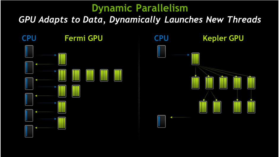
Our parallel implementation mostly follows the same process as our sequential version, the only real differences are we now need to change the code so that it can be run on the GPU. To do this we are going to use CUDA C/C++. 

Like before the first thing we need to do is create variables for holding our three grids and allocate the memory for them on the GPU.


Once we have this we then create a temporary variable on the CPU which we use to initialise all the values in the grid to zero and set our initial goal values. Again we use the centre tile in the grid and set the value to 1024. We then copy our temporary variable from our CPU into our three variables stored on the device.

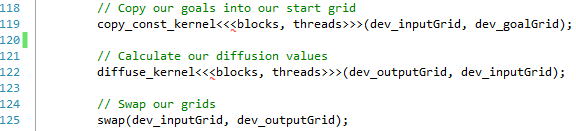
After all our memory is set up on the GPU we can now call our kernels to run our diffusion process. Like the sequential version we follow the same three steps as before. First we copy our goals into our input grid (Line 119). Secondly we calculate our new diffusion values (Line 122) and finally we swap our input and output grids ready for the next iteration (Line 125). 


Our copy_const_kernel follows the same idea as setting our goals did in the sequential version. However this is where the power of parallelization begins to come in as we now no longer need to loop through our entire grid, instead we simply find which tile in the grid the thread is working on and check to see if that tile contains a goal value. If it does we set the goal at this position in the input grid. 


The diffuse_kernel again works in a very similar way, we find the tile we are working on and then get the diffusion values for the left, right, top and bottom neighbours before computing an average and setting this to the value of the corresponding tile in the output grid. 


Finally we swap our input and output grids using the swap() method from the C++ library like we did before.

The final step we need to take into consideration when programming for the GPU is getting our values back onto the CPU once we are finished processing. After we have run our diffusion process for our desired number of iterations we can now pass our data back and store it again in our temporary variable and use it in anyway we wish. 


Time Differences


Overall there is not much difference from our sequential version in terms of the process that we follow and even the amount of code that we have to write. The biggest difference between the applications only becomes noticeable when we start to measure the performance.  

For each of the applications we have measured the time taken to run one iteration of the diffusion process, this involves copying our goals into the input grid, calculating the new values and swapping the input and output grids. This process has been run 100 times and an average time has been taken. 

The applications have been run on grids of 32x32, 64x64, 128x128, 256x256, 512x512, 1024x1024 and 2048x2048.  


Looking at the timings for the different grid size of the sequential version we can see that as the grid size increases so does the time taken to process all the nodes, starting at 0.73ms for a 32x32 grid and moving up to 3 seconds for a grid size of 2048x2048.

Initially this doesn't seem to bad at first glance but we need to remember that we cant find paths from everywhere in our grid until the 'scent' of our goal has spread to every tile. Based upon testing with the parallel implementation it takes at least 40,000 iterations to fill the entire grid so that every tile has a non zero value for a grid of size 2048x2048, This would mean it would take at least 33 hours before we could find all our paths! Ain't nobody got time for that! 


Looking at our parallel times we can see that it follows the same trend as before with our larger grids taking more time to process. However when we look at our actual times we can see a massive difference in speed compared to our sequential versions. 

For our parallel implementation it only takes us 2.44 ms to run our diffusion process for the 2048x2048 grid compared to the 3000 ms of the sequential version. This is also faster than the sequential version for the 64x64 grid even though the 2048x2048 grid is 32 times larger in size! 

This also means that we are able to find all paths to our goal a lot quicker in parallel for our 2048x2048 grid. Considering that it takes at least 40,000 iterations so that all tiles have a non zero value it would only take 97 seconds to find all paths in parallel compared to 33 hours if we done it sequentially. Although still not quite real time it is a lot better! 

Saturday 9 November 2013

Pathfinding Using Collaborative Diffusion

For my honours project this year at university i am aiming to compare pathfinding algorithms on the GPU, One of the algorithms i have chosen to compare is collaborative diffusion so i have implemented a simple application in which agents seek out food items within a maze using the collaborative diffusion algorithm to find the quickest path to the nearest item. The yellow cubes represent the agents, green spheres are food objects and orange cubes are walls which are impassable.

Collaborative Diffusion Explanation

Traditionally in a game each agent will have its own pathfinding routine that will be called any time an agent needs to find a path to a specific goal state. Typically in the majority of games this will call the A* algorithm, this works well in most cases but as the number of agents increases the time spent pathfinding also increases which can have a detrimental effect on the performance of the game.

To combat this collaborative diffusions works on the idea of antiobjects, an antiobject is a type of object that appears to do the opposite of what we would generally think the object would be doing (Repenning, 2006).  For example in the game Pac man (Pac-Man, 1980) the objective of each ghost is to find Pac man. Using traditional pathfinding like A*, each ghost would run its own pathfinding algorithm every time it needed a new path. From an object orientation stand point this makes sense to many programmers that the responsibility of finding a path would be down to each agent, however by removing the computation from the objects that typically appear to do the search, it allows the computation to be redistributed in a parallel fashion to the objects that define the space to be searched instead.

Diffusion is a gradual process in which physical and conceptual matter, such as molecules, heat, light, gas, sound and ideas are spread over an N-dimensional physical or conceptual space over time (Repenning, 2006), within collaborative diffusion this idea is used to transfer the scent of a goal state throughout the world in which pathfinding will be taking place. This diffusion value is calculated using the following equation.
Where:
D = diffusion value
n = number of neighbours
a = diffusion value of neighbour.

Typically the world is organised as a grid representing either a 2D or 3D environment and each neighbour is defined according to the Moore neighbourhood (Moore Neighbourhood, 2013) which comprises of the eight cells surrounding a central cell.

Each goal state is given an initially high diffusion value which is used as the starting state as shown by the green tile in Figure 2 below.

Figure 2 - starting state

During the first iteration the diffusion value for all the tiles are calculated using the diffusion equation. After this iteration the tiles surrounding the goal state now have a larger diffusion value than they had initially and the ‘scent’ of the goal state is beginning to move toward the agent as shown in Figure 3 below.

Figure 3 - Iteration one

This process continues again for all of the tiles in the world during the next iteration, as the diffusion value is calculated again for all the tiles it begins to spread out further from the goal state expanding the ‘scent’ of the goal further across the grid and towards the agent. During this iteration the diffusion value of the tiles surrounding the goal state becomes larger making the goal state appear more attractive to an agent. This second iteration is shown in Figure 4 below.

Figure 4 - Iteration two

At each iteration the diffusion process repeats expanding further and further outwards across the tiles. Eventually the ‘scent’ produced by the tiles will reach an agent at which point a path can be found to the goal state.

Once the ‘scent’ has reached the agent, it is possible for a path to the goal state to be found, unlike pathfinding algorithms like A* which use a back tracking algorithm to find a path from the starting state to the goal state all the agent simply has to do is look up the diffusion values of the tiles neighbouring the tile it is currently on and move to whichever one has the highest diffusion value.

As shown in Figure 5 during the third iteration our agent is able to pick up the ‘scent’ of the goal state, by simply moving to the neighbour with the highest diffusion value our agent is able to find the quickest path to the goal as represented by the green tiles.

Collaborative diffusion allows agents to collaborate together to complete objectives in a very simple manner. In his paper collaborative diffusion: programming antiobjects, Alexander Repenning states that there are four different types of agents that allow collaboration to occur:
  • 1      Goal Agents: Goal agents are pursued by other agents and can be either static or mobile.

  • 2      Pursuer Agents: A pursuer agents is an agent that is interested in one or more of the goal agents. Multiple pursuer agents may be interested in the same goal and may collaborate or compete with one another.

  • 3      Path Environment Agents: A path environment agent allows pursuer agents to move towards a goal agent and participates computationally in the diffusion process. In a simple arcade game this could be a floor tile in a maze.

  • 4      Obstacle Environment Agents: Work in a similar manner to path environment agents but rather than helping an agent to reach the goal they interfere with the agents attempt to reach a goal. This could be represented by a wall or obstacle in a room.

Making use of these different types of agents Repenning noticed that agents would appear to collaborate with one another to reach a goal. He also states that the collaboration between the agents is an emergent behaviour as no code is explicitly responsible for orchestrating a group of agents but is instead a result of the diffusion process and the way in which pursuer agents find a path to goal agents through the path environment agents. Another interesting observation by Repenning is that as the number of agents is increased the time taken to perform the pathfinding remains constant (Repenning, 2006).

By its very nature collaborative diffusion lends itself very well to a data parallel implementation on the GPU, as the GPU works by splitting the work across a number of threads and having each thread perform the same task it should be more than possible to split the work of the tiles across a number of threads as each tile performs the same diffusion calculation.


Bibliography


Pac-Man. (1980). Retrieved October 26, 2013, from Pac-Man: http://pacman.com/en/pac-man-history/


Repenning, A. (2006). Collaborative Diffusion: Programming Antiobjects. Boulder: University of Colorado.